Double Spring in Haskell

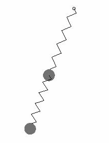
This is an attempt to simulate a double spring model using 4th order Runge-Kutta simulation in Haskell. The model consists of two springs where the first is fixed at one location. At the bottom of the first spring a point mass is located. Attached to the first mass is a second spring which ends in a second point mass.

At first my model seemed to be unstable when the mass was above the spring. Finally I realized that this was due to an erroneous calculation of the angle (phi) from the location of the masses (x1, y1, x2, y2). atan has two solutions (separated by pi) where only one is valid. I had to add pi (via addPi function) to handle that case.

The haskell code for Runge-Kutta is largely taken from Runge-Kutta with Haskell, but I have changed the algorithm to match the following algorithm instead, 16.1 Runge-Kutta Method. gloss is used to output graphics.

The haskell code is shown below.

module Main (main) where
import Graphics.Gloss
import System.Random

{- "(Double) Spring Pendulum" 
   See: http://www.myphysicslab.com/dbl_spring2d.html
   Compile: ghc -O2 SpringPendulum.hs
   Optimize: strip SpringPendulum -o SpringPendulum
   Run: ./SpringPendulum -}
   
instance (Num a) => Num [a] where
  (+) = zipWith (+)       -- e.g. [a,b]+[c,d]=[a+c,b+d]
  negate = fmap negate
  fromInteger = undefined
  (*) = undefined
  abs = undefined
  signum = undefined

-- One iteration of runge kutta. Calculate y(t+h) from y(t)
-- f'(y) is system derivate, h step length and y current state, y(t)
-- See: http://tnt.phys.uniroma1.it/twiki/pub/TNTgroup/AngeloVulpiani/runge.pdf
rk4 :: (Functor f, Floating a, Num (f a)) => (f a -> f a) -> a -> (f a) -> (f a)
rk4 f' h y =
  let
    (.*) n = fmap (*n)
    shf = ((1/2).*)
    k0 = h .* (f'   y)           
    k1 = h .* (f' $ y + shf k0)
    k2 = h .* (f' $ y + shf k1)
    k3 = h .* (f' $ y + k2)    
  in
    y + (1/6) .* (k0 + 2 .* k1 + 2 .* k2 + k3)

-- Integrate system using runge kutta approximation
integrate :: (Functor f, Floating a, Num (f a)) => (f a -> f a) -> f a -> a -> [f a]
integrate f' y0 h = iterate (rk4 f' h) y0

-- System derivate, f'(y), for two masses (m1, m2) where m1 is connected to origo through spring
-- with k1 coefficient. m2 is connected to m1 through spring with k2 coefficient
-- See: http://www.myphysicslab.com/dbl_spring2d.html
double_spring m1 m2 k1 k2 r1 r2 g (x1:y1:x2:y2:v1x:v1y:v2x:v2y:_) = 
  [ v1x, v1y, v2x, v2y, 
    (-1)*(k1/m1)*s1*sin(phi1) +      (k2/m1)*s2*sin(phi2),
    (-1)*(k1/m1)*s1*cos(phi1) +      (k2/m1)*s2*cos(phi2) + g ,
                                (-1)*(k2/m2)*s2*sin(phi2)     , 
                                (-1)*(k2/m2)*s2*cos(phi2) + g   ] 
  where
    l1 = sqrt(x1^2+y1^2)
    l2 = sqrt((x2-x1)^2+(y2-y1)^2)
    s1 = l1-r1
    s2 = l2-r2
    phi1 = atan(x1/y1) + addPi y1
    phi2 = atan((x2-x1)/(y2-y1)) + addPi (y2-y1)

-- Helper converting radians to the degrees used by gloss
radiansToDegrees :: Float -> Float
radiansToDegrees r = (-360)*(r/(2*pi))

-- Helper used when determining the angle from atan(a/b)
addPi b = if (b>0) then 0 else pi

-- Show a mass m on a spring from p1 to p2
showSpring :: Float -> Float -> Point -> Point -> Picture
showSpring m r0 (x1,y1) (x2,y2) = 
    pictures $ [ spring (round r0) (x1,-y1) (x2,-y2), Translate x2 (-y2) $ Color c $ ThickCircle r 1 ]
    where
      sphere_radius vol = (vol*3/(4*pi))**(1/3)
      r = sphere_radius m
      c = light $ light black

-- Show spring from p1 to p2 n is rest length
spring :: Int -> Point -> Point -> Picture
spring n (x1,y1) (x2,y2) = Translate x1 y1 $ Rotate (radiansToDegrees phi) $ Scale (l/r) 1 $ Line ps where
    (dx,dy) = (x2-x1,y2-y1)
    r = fromIntegral n              -- rest len
    l = sqrt(dx^2+dy^2)             -- actual len
    phi = atan(dy/dx) + addPi dx    -- angle
    xs = [0, 0.25 .. r]
    ys = take (length xs) $ concat $ repeat [0,0.5,0,-0.5]
    ps = zipWith (\x y -> (x, y)) xs ys

main = do
  let h = 0.001
  let total_time = 20*60
  let (r1, r2, m1, m2, k1, k2) = (5, 5, 0.1, 0.1, 1,1)
  let (x1, y1, x2, y2) = (5, 0, 10, 0)
  let series = take (floor (total_time/h)) (integrate (double_spring m1 m2 k1 k2 5 5 9.81)  [x1,y1,x2,y2,0,0,0,0] h)
  c <- getChar
  animate
    (InWindow "Double Spring" (400, 400) (150, 150))
    white
    (doubleSpring m1 m2 r1 r2 h series)   -- function of t that produce the picture

-- Produce picture from constants and pre-calculated model-data (series)
doubleSpring m1 m2 r1 r2 h series t = Translate 0 trans $ Scale scale scale $ picture
  where   
    size = 400
    scale = 15
    trans = 0.4*(fromIntegral size)
    picture = showSystem (series !! (floor (t/h)))   
    showSystem (x1:y1:x2:y2:v1x:v1y:v2x:v2y:_) = pictures $ [ ThickCircle 0.2 0.1, 
                                                              showSpring m1 r1 ( 0, 0) (x1,y1),
                                                              showSpring m2 r2 (x1,y1) (x2,y2) ]

A movie of the simulation can be found below.

Try out the hamilton library

Try the hamilton library for this purpose.

Try out the ad library

Try the ad library for this purpose.